Overview

The grey hematite Martian analog sample exhibited a dielectric relaxation loss that was frequency and temperature dependent. Frequency dependence was modeled by fitting the Cole-Cole parameters. Temperature dependence was modeled using a generalized Boltzmann temperature dependence. The generalized Boltzmann temperature dependence was then inserted into the Cole-Cole model to estimate the material EM properties as a function of both frequency and temperature. The dielectric permittivity values were normalized to a density of 1.60 g/cm³ using Equation 1 [Olhoeft and Strangway, 1975].

where:
ε_r^* = complex relative dielectric permittivity

d = density

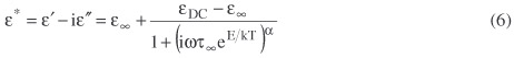
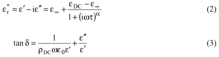
Frequency Dependence

To model the frequency dependence of the grey hematite sample at each temperature, the data were inverted to determine the best fit model parameters of the Cole-Cole equation, Equation 2 [Cole and Cole, 1941]. The Cole-Cole equation assumes a log-normal probability distribution for the time constant of relaxation, Ä [Cole and Cole, 1941]. The time constant of relaxation represents the period of the frequency where the maximum relaxation occurs, which also corresponds to the maximum value of µ". Equation 3 is the total electrical loss tangent. The resistivity of the grey hematite was so large it could not be measured.

where:
ε′ = real part of the relative dielectric permittivity

ε″ = imaginary part of the relative dielectric permittivity

ε_∞ = relative dielectric permittivity at infinite frequency

ε_DC = relative dielectric permittivity at low frequency

ω = angular frequency

= time constant of relaxation

α = distribution parameter

tan δ = total electrical loss tangent

ρ_DC = DC conductivity

ε₀ = dielectric permittivity of vacuum = 8.8541×10^-12 F/m

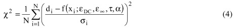
Inversion was used to determine the value and confidence intervals for each of the four Cole-Cole parameters (ε_DC, ε_∞, , α) that best fit the averaged data. Similar data had been inverted before using a Levenberg-Marquardt routine [Canan, 1999]. However, that data had a larger bandwidth and contained higher losses. A similar inversion routine was programmed utilizing MATLAB^®'s Optimization toolbox. This program also used a Levenberg-Marquardt [Levenberg, 1944, and Marquardt, 1963] inversion to find the global minimum of a weighted normalized chi squared fit, Equation 4, of the Cole-Cole equation.

where:
= data to model misfit

d = data

f = Cole-Cole equation

x = modeled data points

N = number of data points

σ = standard deviation

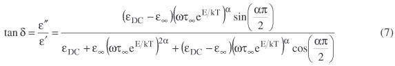
Once the global minimum was found, two adjusted data sets were created by adding and subtracting a standard deviation from the original averaged data set. Adjusted chi squared values were found for each of the adjusted data sets with the previous best fit model. The model parameters were then varied individually to match the adjusted chi squared value. This gave the 95.5% confidence intervals for each parameter, see Figure 1. The inversion process was applied to the data collected at the coldest temperature (180.9K) first, because it contained the largest portion of the relaxation. Next the remaining temperature data sets were inverted with three of the Cole-Cole parameters (ε_DC, ε_∞, α) constrained by their 95.5% confidence intervals found in the coldest temperature (180.9K) fit. Lastly, the 95.5% confidence intervals were found for each data set s fourth parameter, time constant of relaxation (τ). Figure 2 shows the fit of the inversion to the grey hematite data for three temperatures.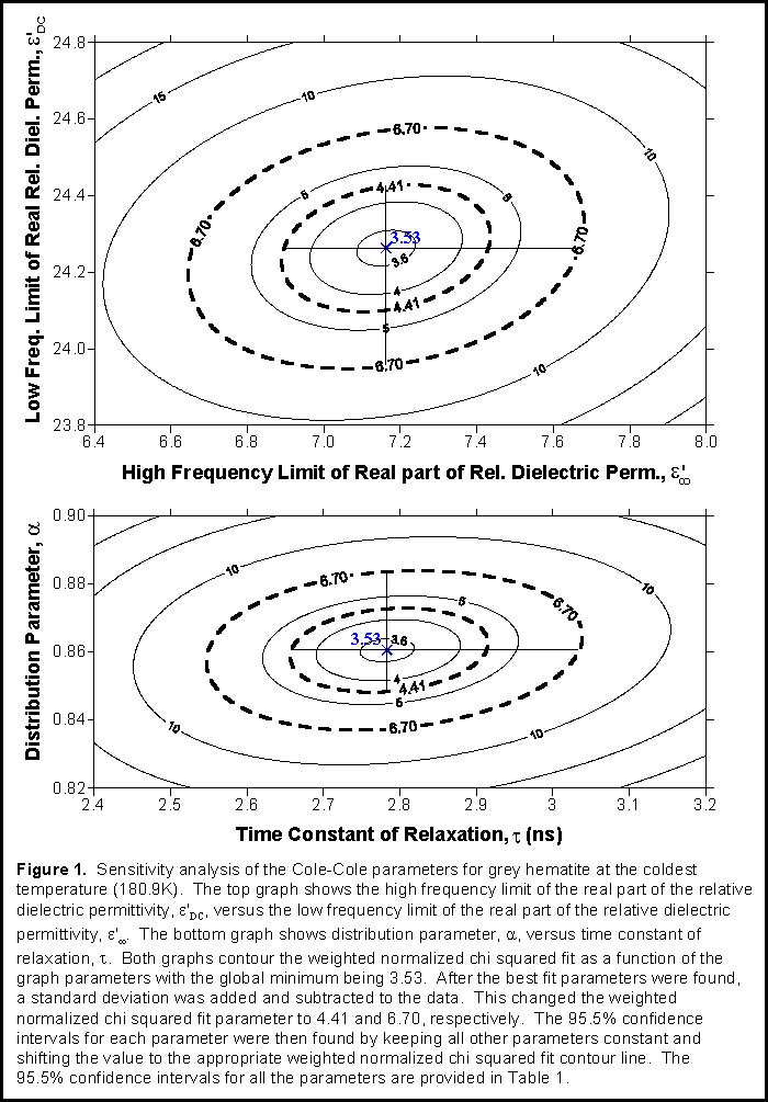

Temperature Dependence

From the inversion results, it was found that the time constant of relaxation, , increased as temperature decreased. This variation in time constant of relaxation with temperature was modeled by a generalized Boltzmann temperature dependence [Olhoeft, 1976], Equation 5. The generalized Boltzmann temperature dependence assumes a Maxwell-Boltzmann distribution of the process causing the temperature dependent dielectric relaxation.

where:
_∞ = time constant of relaxation at infinite temperature

E = activation energy

k = Boltzmann s constant = 8.6176×10^-5 eV/K

T = temperature, K

Figure 3 shows an Arrhenius plot of the time constant of relaxation versus the inverse product of temperature and the Boltzmann constant, as well as the best fit line. The time constant of relaxation error bars are the 95.5% confidence intervals and the horizontal error bars represent the accuracy of the temperature values with respect to thermistor accuracy (±0.2K when greater than 193K and ±2K when lower than 193K). The confidence intervals of the time constant of relaxation at infinite temperature (zero crossing on Fig. 3) and activation energy (slope of the line on Fig. 3) were found by fitting a separate line with the data points shifted to one extreme limit of their individual confidence intervals to acquire a range of best fit lines.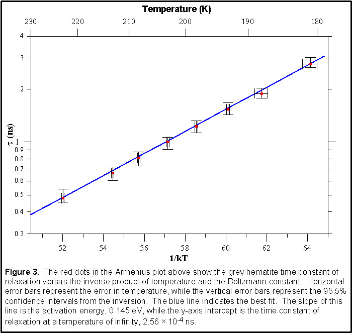

Temperature and Frequency Dependence

After the time constant of relaxation was modeled with the generalized Boltzmann temperature dependence as a function of temperature, it was inserted into the Cole-Cole equation (Equation 6) and electrical loss tangent equation (Equation 7). The values in the lossy table were normalized to a density of 1.60 g/cm³ using Equation 1, and then substituted into Equations 6 and 7 to describe how dielectric permittivity and electrical loss tangent vary with frequency and temperature.

Currently, two orbital radars are planned to probe into the subsurface of Mars. MARSIS, located on Mars Express, has four frequency bands centered at 1.8, 3.0, 4.0, and 5.0 MHz with a bandwidth of 1 MHz [Safaeinili et al., 2001]. SHARAD, which will fly on Mars Reconnaissance Orbiter, has one band centered at 20 MHz with a bandwidth of 10 MHz that can be split into two frequency bands centered at 17.5 and 22.5 MHz with a 5 MHz bandwidth [Seu et al., 2004]. Both SHARAD and MARSIS have a dynamic range of 50-55 dB [Safaeinili et al., 2001], [Seu et al., 2004]. Figure 4 is a graphic representation of the lossy table with MARSIS and SHARAD frequency bands included.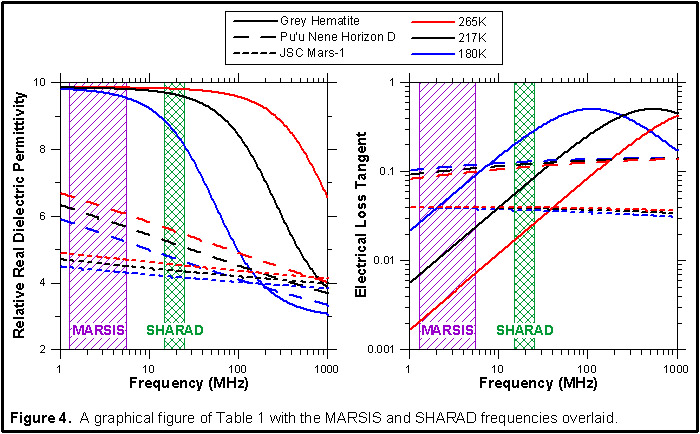

Polarization Mechanism

Dielectric relaxations occur when the internal charges of a material can no longer move fast enough to fully separate before the external field switches polarity. The frequency column in the table below lists the maximum frequency at which various mechanisms for charge separation can respond.

The polarization mechanism causing the temperature dependent dielectric relaxation in the grey hematite sample occurred at 2.12 GHz at room temperature (298K) with an activation energy of 0.145 eV. Ionic and orientation polarization mechanisms did not take place in the sample since it was dry and contained no surface charges. Electronic polarization did occur in the grey hematite sample. However, this mechanism is frequency independent in the radar frequency. The most likely mechanism that caused the grey hematite relaxation at 2.12 GHz (at 298K) was a molecular polarization mechanism, where internal charges in the grey hematite crystal structure distorted to polarize against an external electric field.

The activation energy determines how the time constant of the molecular relaxation varies with temperature. More specifically, the activation energy represents the energy of the barrier that the charges must overcome in order to become polarized. However, even if an atom has enough energy to become polarized, it still must have enough time to separate before the field changes.

        

Hematite possesses a Morin temperature of 263K. Above the Morin temperature, hematite is in a canted antiferromagnetic state with a magnetization saturation value of 0.4 Am²kg^-1. Below the Morin temperature, hematite changes to an antiferromagnetic state and does not have a magnetization saturation value [Dunlop and Ozdemir, 1997].

  

Based on modeling results, GPR should be able to detect a change in attenuation, velocity, and reflectivity as a result of temperature variations in areas containing grey hematite. A change in reflectivity would be caused by the contrast in dielectric permittivity. MARSIS will not be sensitive to annual or diurnal temperature variations in grey hematite areas. However, SHARAD, due to its higher frequency, will not be sensitive to diurnal variations but may be sensitive to annual variations. A Martian lander equipped with GPR has the best opportunity to see these temperature changes. A higher frequency GPR would only be able to distinguish both diurnal and annual variations, while a lower frequency GPR would only be sensitive to annual temperature variations.