Measurement System

Dielectric permittivity and magnetic permeability measurements are made in the frequency domain using an HP 8753D vector network analyzer (VNA) with a coaxial waveguide sample holder (the setup is shown in figure 1). Custom software run on an external computer controls the VNA and measurements are made from 30 kHz - 3 GHz. The VNA is connected to a pair of 7mm phase matched coaxial cables via its two ports. These phase matched cables are each connected to GenRad 7mm to 14mm adapters (GR-900) which are then both connected to a GR-900 coaxial waveguide sample holder. Three different lengths (3, 5, 10 cm) of sample holders were used in this study. Different sample holders were used to fine tune the accurate frequency reading (discussed in detail below). The EM properties of the waveguide change when a sample is loaded into the coaxial waveguide. To find the EM properties of the sample, one port of the VNA sends a continuous voltage wave down the center conductor of the coaxial line. Since the outer conductor is grounded this voltage wave creates a changing electric field, which then produces a changing magnetic field, shown in figure 2. As the TEM wave travels from the GR-900 adapters to the sample holder a reflection occurs because the impedance of the sample holder is no longer equal to the adapters. Some of the TEM wave travels through the sample holder but at a slower speed. As the TEM wave exits the sample holder to the other GR-900 adapter another reflection occurs. The amount of energy that is reflected and transmitted is expressed as scattering (S) parameters. Figure 3 shows a flow chart on how the S parameters are defined. Equations 1 and 2 are the S parameter equations from the figure 3 flow chart. To find the S parameters one measures at b₁ or b₂ while a₁ or a₂ (This description of how the network analyzer works is borrowed from (Adams, 1969, Baker-Jarvis, 1993, Nicolson and Ross, 1970, Weir, 1974). Once the S parameters have been found they can be converted into the complex EM properties of the material. This is done by understanding what the S parameters represent as seen in Equation 3 and 4 and if Figure 4 as a flow chart.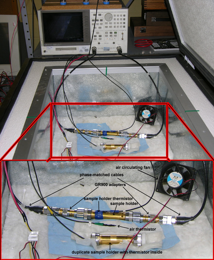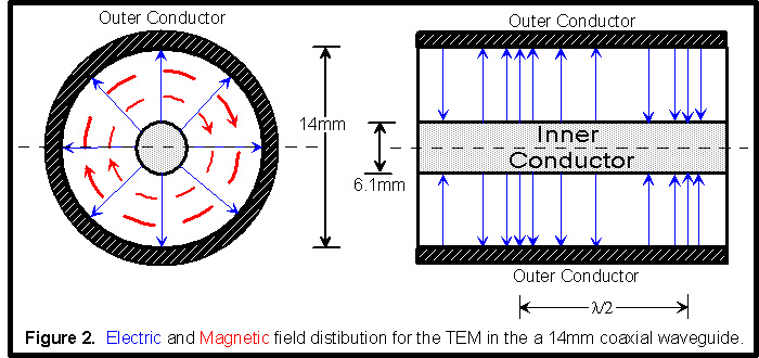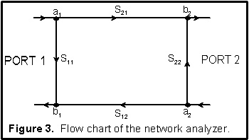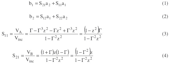

where:
S₁₁ = scattering coefficient orginated at port 1 and measured at port 1

S₂₂ = scattering coefficient orginated at port 2 and measured at port 2

S₂₁ = scattering coefficient orginated at port 2 and measured at port 1

S₁₂ = scattering coefficient orginated at port 1 and measured at port 2

Γ = reflection coefficient

z = transmission coefficient

Equations 5 and 6 define what the reflection and transmission coefficients equal.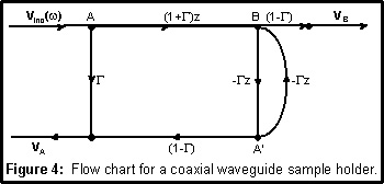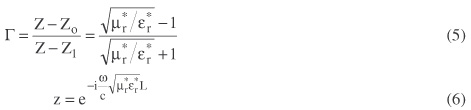

where:

L = length of the sample holder

c = the speed of light

ε_r^* = complex relative dielectric permittivity

μ_r^* = complex relative magnetic permeability

Since the reflection and transmission coefficients equal complex magnetic permeability and complex dielectric permittivity the S parameters equations 3 and 4 are then solved to equal the reflection and transmission coefficients. This is shown in Equations 7-11.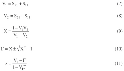

Equation 12 is equation 5 rearranged while equation 13 is 6 rearranged. Equations 12 and 13 are then manipulated in equations 14 and 15 to find the complex EM properties.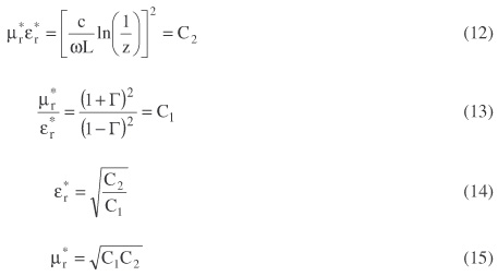

Calibration of VNA

Prior to measuring the sample, the VNA and associated cable connections are calibrated. This process will consist of measuring the reflection of open, short, and load terminators at the end of each of the phase matched cables. Then connecting the two phase matched cables together and measuring the through and reflected response. Then the adapters are added and the reflection of open, short, and load terminators are measured. An empty sample holder is then connected to the adapters and the through and reflected responses are measured. The response of an open, short, and load terminators are shown in figure 4. The responses of a through and reflected measurement are shown on figure 5. To check the calibration, an empty sample holder was measured first. If the test of the empty sample holder showed no losses with a relative dielectric permittivity and relative magnetic permeability of 1, then the calibration was considered successful and the VNA was ready for use. The VNA had to be recalibrated daily if the cables were moved and when multiple samples were measured. If the cables were not moved and the room temperature stayed within ±5K, then the calibration could last for days or possibly weeks.

Temperature Measurements

Before making a VNA measurement, the samples were dried in a vacuum chamber at 3*10^-4 mbar until no appreciable change in weight was measured (0.005% in 24 hours). A sample was then loaded into a 3, 5, or 10 cm long GR-900 sample holder and connected to the VNA. EM measurements were acquired by placing the sample holder in an insulated So-Low Ultra-Low freezer, Model #C85-5, and varying the temperature from 300K to 180K in intervals of 5K or 10K. Three YSI 44006 Epoxy-Encapsulated thermistors were placed in the freezer, one at the bottom of the freezer, one on the outside of the sample holder, and one inside a duplicate sample holder that was packed with the same material and placed next to the actual test sample holder. The temperature of the freezer was then adjusted to the specified temperature. A measurement was taken once the temperature in the duplicate sample holder was within 5% of the target temperature for approximately 15 minutes.

Quality Control

In order to test the suitability of conducting measurements in the freezer, two quality control experiments were conducted using both an empty or air sample and a dry quartz sand sample. During both quality control tests, a VNA measurement was made every 10K from 298K to 193K. Figure 1 shows that the results from the measurements confirmed that accurate data could be acquired at the low temperatures. However, the data did reveal minor problems with cable contraction at the lower temperatures. This error increases when a shorter sample holder is used because the magnitude of the cable contraction is a higher percentage of the sample holder length.

Output of the VNA

The VNA output consists of two data sets with four S parameters (S₁₁, S₁₂, S₂₁, and S₂₂) versus frequency (30 kHz - 3 GHz). The first subscript of the S parameter describes the port of the network analyzer where the signal originated, while the second subscript describes the port where the signal was measured. The amplitude and phase of the four S parameters were measured at each frequency. From the four S parameters, two data sets, from measuring the sample holder in both directions, of real part of the relative dielectric permittivity, real part of the relative magnetic permeability, electrical loss tangent, and magnetic loss tangent were calculated (Canan, 1999). If there is negligible noise, these two data sets should be identical. When the data are not identical, it is typically the result of a heterogeneous sample pack, usually produced by compacting the soil more on one side of the sample holder than the other. Data from the VNA were truncated to remove low frequency noise, instrument artifacts, and resonance effects. Below 100 kHz, the wavelength of the EM energy is much larger than the sample holder and therefore the data are not accurate. At four different frequencies, instrument artifacts cause large data spikes. These are removed as well. At high frequencies, sample holder resonance dominates the data and is removed above the frequency determined by the following equation (Canan, 1999).

When measuring a lossless media (air) with the VNA, nonzero loss tangents are measured. These nonzero loss tangents are not real and considered to be the noise floor of the system. In all loss tangent figures, the noise floor indicates the minimum loss tangent that can be measured. At lower frequencies where the noise floor is decreasing proportional to the frequency, the noise floor is controlled by the conductivity of the sample holder. At higher frequencies where the noise floor is proportional to the frequency, the noise floor is controlled by the resonance phenomenon as well as scattering from scratches along the sample holder. The noise floor at both low and high frequencies is divided by the real part of the dielectric permittivity because it represents loss tangent. After truncation, the two data sets were averaged together and smoothed by a centrally located five-point moving average filter. A standard deviation was calculated for each data point in this same process. If the standard deviation was less than 10% of the average, the data point was removed, this was done to remove even more of the low frequency data. These steps were taken not only to filter the data, but also get the data in a form so that it could be inverted. The inversion processes is discussed here.